Development of an alcohol biosensor non-wear algorithm: laboratory-based machine learning and field-based deployment

Introduction

Alcohol biosensors are capable of continuously and passively recording transdermal alcohol concentration (TAC), a perspired biomarker useful for detecting alcohol consumption^1,2,3,4,5 and severe intoxication^6,7,8. In the past decade, novel wrist-worn alcohol biosensors (e.g. BACtrack Skyn, first released in 2016) have reduced concerns about social stigma, physical discomfort, and low sampling rates associated with older alcohol biosensors, such as the SCRAM CAM ankle monitor commonly used in the judicial system^1,2. Given the predictive validity and established acceptability of wrist-worn biosensors, these devices have the potential to ameliorate high-risk drinking events by facilitating timely delivery of medical assistance⁹.

Before deploying wrist-worn biosensors for just-in-time interventions, signal processing systems must be able to reliably detect when the device is not worn. Wrist-worn alcohol biosensors are typically detachable and require charging, so individuals may avoid wearing or forget to wear the device. Whereas a powered-off device results in missing data, a powered-on device that is not firmly applied to the wrist (i.e., non-wear) results in readings that do not accurately reflect TAC. During non-wear, the biosensor may produce TAC readings that hover around zero, a false positive signal if exposed to environmental alcohol, or an unstable TAC signal if the device is loosely worn during a drinking event¹⁰. When left unaddressed, these muted or noisy signals lead to misclassifications of whether individuals consumed alcohol, diminishing the utility of using TAC features as model outcomes or predictors. However, if non-wear can be precisely detected by an algorithm, data quality can be improved through identification, removal and imputation^3,11,12. Further, a non-wear detection algorithm could be incorporated into real-time smartphone notifications to remind participants to equip or tighten the device, leading to greater adherence and fewer missed drinking events in both natural environment studies and medical interventions.

Without an established non-wear algorithm, prior analyses of Skyn-derived TAC have probed for non-wear by visually assessing plots of temperature¹ or flagging biosensor readings below certain temperature cutoffs (26 °C⁴, 28 °C³, 29 °C²). Temperature cutoffs are straightforward but imprecise, with lower cutoffs overestimating and higher cutoffs underestimating biosensor adherence. A single temperature cutoff does not account for the natural variation in surface body temperature nor the sensor’s temporal delays following device removal or re-application (i.e., temperature readings gradually fall following device removal and gradually rise following device re-application)^13,14. Therefore, to determine whether the device was worn during a particular biosensor reading, algorithms should evaluate temperature at that instance and systematic temperature trends before and after that instance. Further, motion readings recorded by the Skyn may also provide valuable information for algorithm decisions, yet motion and temperature features have not been used together to detect Skyn non-wear. Motion values are likely to be lower during non-wear than wear, especially when the device is resting on a stationary surface (versus, for example, in a backpack or pocket). Intervals of motionlessness might help an algorithm detect non-wear when temperature features are insufficient, such as in warm climates where ambient temperature can resemble body surface temperature¹⁰.

Guidance on non-wear algorithms can be found in work with other biosensors, such as accelerometers^{13,14,15,16,17,18}. In an analysis comparing several published non-wear algorithms, the top-performing algorithm included both temperature and motion time-series features, and it successfully identified 95% of wrist-worn accelerometer non-wear. Despite strong performance overall, for non-wear intervals less than an hour in duration, this algorithm only captured 66% of non-wear. The algorithm’s limited ability to detect brief non-wear intervals may be due to the fact that ground truth labels were determined by error-prone plot annotations and self-report field diaries^15,17,19,20. To develop an algorithm sensitive to both short and long intervals of non-wear, it would be important to acquire high-resolution ground truth labels (i.e., minute-by-minute readings labeled “wear” and “non-wear” with near-perfect accuracy). One way to achieve this is by conducting a laboratory procedure that includes brief, scheduled non-wear intervals^21,22,23. To our knowledge, this approach has not been used previously to develop an algorithm for detecting TAC sensor non-wear.

The goals of the present work were to develop an algorithm that differentiates alcohol biosensor wear from non-wear using laboratory-based ground truth (Study One) and use the algorithm to retrospectively assess biosensor adherence in a separate field study (Study Two). For Study One, we hypothesized that, relative to temperature cutoffs, the newly developed algorithm would show better sensitivity to detect non-wear and better specificity to confirm wear. For Study Two, we hypothesized that the algorithm would agree more with self-report than with a temperature cutoff; we also used algorithm predictions to quantify biosensor adherence across participants and days, then compared adherence across two device models with different battery capacities. By developing a non-wear algorithm and using it to evaluate adherence in the field, this work addresses a critical issue in the validation of biosensor-based alcohol monitoring.

Study one: non-wear algorithm development using laboratory ground truth

Methods: laboratory study

Participants

Biosensor readings were collected during laboratory sessions from 36 participants (Table 1) enrolled in a larger investigation of subjective and objective responses to a fixed-dose oral alcohol challenge and their associations to future drinking outcomes^24,25,26.

Table 1 Sample characteristics.

Full size table

At a screening visit, participants completed informed consent, verified their identity with a photo ID, provided biological samples (breath, urine, and blood), and filled out surveys on health, alcohol, and substance use^27,28. Participants met the study age criteria (40–65 years old) and were approved by the study physician based on their blood pressure, liver enzymes, medications, and substance/medical history. Full eligibility criteria can be found elsewhere²⁹.

Procedures

All study methods were fully approved by the University of Chicago Institutional Review Board. The study was conducted in accordance with governmental regulations and guidelines set by the Declaration of Helsinki. In brief, participants completed two individual double-blinded beverage administration sessions at the Clinical Addictions Research Laboratory at the University of Chicago. Upon arrival, each participant completed breathalyzer, drug, and pregnancy tests (for females) to ensure safety of participation. On separate study days and in random order, each participant consumed either a 0.8 g/kg alcohol beverage or a placebo beverage within a 15-min period²⁴. Before and several timepoints after beverage administration, participants completed a series of surveys and hand–eye coordination tasks with their non-dominant (biosensor-equipped) hand. Laboratory sessions took place in furnished, windowed rooms with an ambient temperature ranging from 19–24 °C (66–75°F). For completing all study components (screening, laboratory study, and an ambulatory phase beyond the scope of this report), participants were compensated $400 ($250 plus a $150 completion bonus). Additional details on the laboratory protocol can be found elsewhere^{24,25,29,30,31}.

Alcohol biosensor

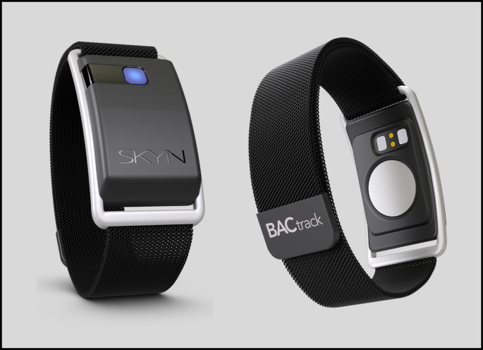
The laboratory study used the BACtrack Skyn (BACtrack, San Francisco, CA, USA), a wrist-worn alcohol biosensor with a magnetic detachable band, a black external housing, a power button, and a small blue light that indicates whether the device is powered on (Fig. 1). On its underside, the device has a charging port and a protective sensor filter. Transdermal alcohol concentration (TAC) is measured by the device via an electrochemical fuel-cell that records micrograms of alcohol per liter of air (μg/L)^32,33. For assessing non-wear, the Skyn measures body surface temperature (degrees Celsius; °C) and motion (acceleration in g-forces; g). The device records TAC, temperature, and motion every 20 s. To upload the data to cloud storage, a smartphone must be connected to the device via Bluetooth and the BACtrack Skyn application must be opened¹⁰. Researchers can then download the raw data from BACtrack’s online research portal. For more information on battery life and data storage, see the Alcohol Biosensor section in Study Two Methods.

Biosensor protocol

Biosensor data were collected during 33 alcohol sessions and 28 placebo sessions. At the start of the baseline timepoint, participants equipped the wrist-worn biosensor to their non-dominant hand. Four unique Skyn devices, all Model T15 with firmware 4.13.1, were used during the laboratory study. These devices recorded data for a range of 44.4 to 73.1 h, totaling 245.0 h of Skyn data.

Ground truth non-wear

There were two a priori determined non-wear intervals during each session at approximately 45 min and 180 min after the onset of beverage ingestion. At each of these intervals, the participant was instructed to remove the device and give it to the research assistant who placed it on a table for about 10–20 min. After this interval, the participant was asked to reapply the device to their wrist. At each instance of device removal and re-application, the research assistant simultaneously recorded the hour and minute to an online database³⁴. Throughout the study, there was a total of 120 non-wear intervals. See Fig. 2 (or Supplemental Fig. S1) for the device removal protocol and corresponding changes to temperature and motion.

Data were downloaded from the BACtrack research portal at one reading per minute (rather than one reading per 20 s) to simplify time-series interpretation and minimize data processing burden, consistent with prior work^3,4. Using ground truth timestamps recorded by research assistants, every biosensor reading was labeled “worn” or “not worn”. Per session, based on ground truth labels, the device was worn for an average (± standard deviation) of 189.9 ± 20.0 min and not worn for 51.1 ± 13.3 min. Variation in wear and non-wear durations was due to varying rates of timepoint completion and minor procedural deviations (two sessions missed the first scheduled removal and nine sessions included removal at the end rather than the start of the 180-min timepoint). These deviations proved to be minimally consequential, as timestamps of non-wear intervals were still recorded and used to label ground truth for these sessions, resulting in more robust training data via increased variability of non-wear intervals.

Algorithm development

Algorithm features

A random forest algorithm³⁵ was trained to differentiate between “worn” and “not worn” using temperature and motion recorded by the Skyn, as well as 20 additional features computed from temperature and motion: the difference between the current reading and the prior reading (prior change) and the difference between the current reading and the subsequent reading (subsequent change); the difference between the current reading and the mean of the 10 preceding readings (prior mean change) and the difference between the current reading and the mean of the 10 succeeding readings (subsequent mean change); the quadratic coefficients of the 10 preceding readings and the 10 succeeding readings (i.e., the curvature (a), slope (b), and intercept (c) of y = ax² + bx + c, where x is minutes relative to current timestamp and y is either temperature or motion). In total, the algorithm used 22 continuous features (Table 2).

Table 2 Feature importance rankings of the random forest algorithm.

Full size table

Because time-series features depended on nearby values for their computation, time-series features were not computed when there were 5 or fewer available nearby readings. Limited nearby readings occurred before and after the laboratory session when the device was powered off. To enable algorithm predictions beside intervals of missing data, we configured three additional random forests: (1) a pre-gap algorithm built without subsequent features, designed to make predictions on data before an interval of missing data; (2) a post-gap algorithm built without prior features, designed to make predictions on data after an interval of missing data; (3) a between-gap algorithm built only with current temperature and motion, designed to make predictions on readings surrounded by missing data. The final non-wear algorithm defaults to the 22-feature random forest, but if certain features cannot be computed due to missing data, the algorithm will utilize predictions from the appropriate reduced-feature algorithm. To assess performance of the final combined algorithm, all available predictions from the 22-feature algorithm were used (which accounted for 99.1% of laboratory data) and predictions from the reduced-feature algorithms were used for the remaining 0.9%.

Training

Each random forest was trained using device-based cross-validation^36,37, also called leave-source-out cross-validation. As there were four unique devices used throughout the laboratory study, the data were split four times such that, at each split, three devices’ data were used for training and one device’s data were reserved for testing. Device-based cross-validation was chosen to evaluate how well the algorithm generalized to discrete devices³⁷ and to limit wasting data as in single-split approaches³⁸. At the conclusion of the fourth split, each device had a turn being left out and every biosensor reading had a corresponding prediction of “worn” or “not worn”. A probability threshold of 0.5 was used to classify wear and non-wear readings. For details on hyperparameter tuning, see Supplementary Table S1.

Performance metrics

Given the precedent set by prior non-wear algorithm research^17,18, non-wear was considered a positive classification. Therefore, correct predictions of non-wear were considered true positives, correct predictions of wear were considered true negatives, incorrect non-wear predictions were considered false positives, and incorrect wear predictions were considered false negatives. From these counts, sensitivity (proportion of detected non-wear), specificity (proportion of confirmed wear), and accuracy were calculated, as well as their 95% confidence intervals (CI) based on the Wilson score method. The area under the receiver operator curve (AUC-ROC) was also calculated. These metrics were calculated separately for each device and collectively for the entire dataset.

Algorithm performance was compared to the predictive performance of five different temperature cutoffs (26, 27, 28, 29, and 30 °C), three of which (26, 28, and 29 °C) have been used in prior research to detect Skyn non-wear^2,3,4. For each cutoff, biosensor readings above or equal to the cutoff were labeled “worn” and readings below the cutoffs were labeled “not worn”. True positives, true negatives, false positives, false negatives, sensitivity, specificity, and accuracy were calculated for each temperature cutoff.

Feature importance

Mean decrease in impurity (MDI) and split selection percentage were calculated for each of the features in the complete 22-feature random forest. MDI provides an indication of relative importance toward predictive accuracy, with larger values indicating greater ability to differentiate wear versus non-wear^35,39. Split selection percentage represents the proportion of all decision splits that incorporated a particular feature. More information on MDI and split selection is provided in Supplementary Table S2.

Code

Data processing and machine learning software was built using the Scikit-learn³⁹ and Pandas⁴⁰ modules in Python. The trained algorithm and temperature cutoffs have been added to the Skyn Data Manager³ as optional strategies for flagging non-wear. To replicate algorithm development, see repository here: https://zenodo.org/records/16914785. For the complete Skyn Data Manager software, access may be granted upon request to the corresponding author.

Results: laboratory study

Sample

The laboratory sample consisted of 36 individuals (18, 50.0% female) with an average age of 50.6 years. Participants were mostly White (n = 31, 86.1%) and consumed an average of 16.4 drinks per week (Table 1).

Temperature and motion descriptives

Throughout the laboratory study, temperature ranged from 20.6 °C to 36.5 °C and motion ranged from 0.004 g to 0.98 g. Based on laboratory ground truth, the average (± standard deviation) temperature and motion were, respectively, 31.2 ± 1.7 °C and 0.11 ± 0.14 g while the device was worn, compared to 25.7 ± 2.5 °C and 0.02 ± 0.04 g while it was not worn.

Temperature cutoff performance

For temperature cutoff predictions in the laboratory, the greatest sensitivity (± 95% CI) to detect non-wear occurred at the 30 °C cutoff (0.934 ± 0.009 CI), but this cutoff had the least specificity to confirm when the device was worn (0.774 ± 0.008 CI). Conversely, the greatest specificity to confirm when the device was worn occurred at the 25 °C cutoff (0.994 ± 0.001), but this cutoff had the worst sensitivity to detect non-wear (0.463 ± 0.018). The temperature cutoff of 28 °C had the highest accuracy of all temperature cutoffs (0.940 ± 0.004), showing strong specificity (0.974 ± 0.003) while also retaining moderate sensitivity to detect non-wear (0.815 ± 0.014).

Algorithm performance

As hypothesized, the algorithm performed with greater specificity and greater sensitivity than each temperature cutoff (Fig. 3). Across the four devices used for laboratory testing, sensitivities ranged from 0.917–0.978, specificities ranged from 0.989–0.999, and AUC-ROCs ranged from 0.998–0.999 (Table 3). Overall, the algorithm demonstrated high sensitivity to detect non-wear (0.960 ± 0.007) and high specificity to detect when the device was worn (0.995 ± 0.001), with an AUC-ROC of 0.999.

Table 3 Non-wear algorithm performance with laboratory ground truth data.

Full size table

Out of the 120 device removals throughout the laboratory study, 119 had at least one concurrent non-wear prediction (i.e., only one removal went entirely undetected). Out of 245.0 h of laboratory data, there were 101 discrete intervals of incorrect predictions, with the average duration being 2.4 min and the longest interval being 24 min. See Supplementary Materials for additional plots (Fig. S2) and results (Tables S3 and S4).

Algorithm feature importance

Out of the 22 algorithm features (Table 2), the four most important were subsequent temperature intercept (MDI = 0.249), temperature (MDI = 0.219), prior mean temperature change (MDI = 0.111), and preceding temperature intercept (MDI = 0.088). While motion features were less important overall than temperature features, motion (MDI = 0.030) was ranked eighth most important. Across all features, split selection percentages ranged from 2.75% to 6.99%. For more results on feature importance, see Supplementary Table S2.

Study two: field-based deployment of non-wear algorithm