Spatial metabolic gradients in the liver and small intestine

In mammals, tissue metabolism is fuelled by circulating nutrients coming from diet or inter-organ exchange^6,7. The small intestine contributes to digestion, nutrient absorption and initial processing of dietary nutrients⁸. The liver processes dietary nutrients and xenobiotics, and regulates systemic carbohydrate, fat and protein metabolism⁹. Together, the intestine and liver shape whole-body metabolic homeostasis.

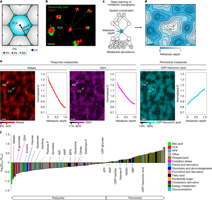
Tissue function depends on its spatial architecture. In the liver, cells are spatially organized into repeating hexagonal lobules^1,2,3. Nutrient-rich and oxygenated blood percolates through lobules from portal nodes at the lobule corners into the draining central vein (Fig. 1a). This spatial arrangement induces nutrient and oxygen concentration gradients along the portal–central axis. Hepatocyte gene expression similarly varies along this axis^2,3,9,10. Such zonation helps the liver in performing a wide range of physiological processes simultaneously, some of which are functionally reciprocal^1,3,9. Spatial gene expression gradients are also observed in the small intestine^5,11. There, differentiated epithelial cells originate in the crypts and migrate towards the villus tips^12,13. Cells along the crypt–villus axis are exposed to concentration gradients of circulating compounds as blood flows from crypts to villus tips (Fig. 2a). Thus, both gene expression and nutrient access may contribute to spatial metabolic organization of liver and intestine.

Metabolic zonation in the liver and small intestine has previously been mostly inferred from gene and protein expression^1,2,5,14,15. However, gene expression does not always reflect cellular phenotype. The spatial distributions of protein and transcript levels are weakly correlated^14,15. Enzyme levels only partially explain metabolic activity¹⁶. Accordingly, direct metabolic measurements are needed. To date, liver metabolomics has been obtained at low spatial resolution (≥30 µm) and without quantification of portal–central gradients¹⁷, with the exception of a few metabolites measured through secondary-ion mass spectrometry, a technique with micrometre spatial resolution but limited metabolome coverage¹⁸. Spatial measurements of intestine metabolic gradients are lacking.

Beyond metabolite abundances, there is value in understanding metabolic activity spatially. Metabolite levels alone do not reflect pathway activity^19,20,21,22, as higher metabolite abundances can be attributed to either faster production or slower consumption. The combination of stable-isotope tracing and IMS hold potential in this regard^23,24,25, but to date has been achieved only at low spatial resolution.

Here we map metabolite abundances and pathway activity at a high spatial resolution using MALDI-IMS (15 µm for liver, 10 µm and 5 µm for intestine). We develop a deep-learning approach that infers from metabolomic images the predominant underlying spatial pattern (metabolic topography). Such analysis revealed that more than 90% of metabolites vary significantly along the portal–central axis in the liver and along the crypt–villus axis in the intestine. We further show metabolic activity patterns underlying these concentration gradients, and local disruption in the levels of perhaps the most fundamental metabolite, ATP, by the obesogenic dietary nutrient fructose.

We collected MALDI-IMS data from mouse liver slices. From the raw data, 156 ions, including those corresponding to deprotonated and other forms (such as sodium, potassium and chloride adducts) of canonical lipids and water-soluble metabolites, were detected across independent mouse liver slices. Of these, 144 were deprotonated ions of canonical metabolites and lipids based on exact mass match and further identity confirmation (natural isotope abundance distribution, tandem mass spectrum and/or isotope labelling; Supplementary Table 1). Across metabolites, MALDI-IMS signals correlated with bulk metabolomics (Extended Data Fig. 1a,b).

A common challenge in IMS is to assign pixels a histological identity, which can sometimes be tackled by co-registering and overlaying spatial information from other imaging modalities^26,27. In the context of liver anatomy, we sought to determine the spatial location of a given IMS pixel along the liver portal–central axis in an automated manner and without the need for other orthogonal imaging approaches. Both portal and central veins could be identified by the presence of haem (Fig. 1b). Portal nodes were further distinguished by the presence of bile ducts as indicated by bile-acid ions (taurocholic acid) (Fig. 1b) and confirmed by histology analysis of the same slide after MALDI imaging and by immunofluorescence (Extended Data Fig. 2a,b).

We hypothesized that the position along the portal–central axis would be the primary spatial metabolic feature in the liver, and that it could be automatically inferred by deep learning. Building from our recently introduced method GASTON for spatial transcriptomics (Methods), we developed a deep-learning method for identifying spatial metabolic gradients (Metabolic Topography Mapper, MET-MAP; https://metmap.princeton.edu/). This approach learns a one-dimensional (1D) coordinate (metabolic depth) in an unsupervised manner (that is, without prior knowledge of tissue anatomy) that best recapitulates the observed high-dimensional spatial metabolomics data (Fig. 1c). Metabolic depth is analogous to contour lines on a topographical map (Fig. 1d). In the liver, it recapitulates the classical hexagonal lobule architecture (Fig. 1d) and correlates strongly with position measured directly along the observable portal–central axes (Extended Data Fig. 2c–g). Thus, in a fully unsupervised manner, metabolic depth defines the liver’s hallmark portal–central organization.

We next examined how metabolite concentrations vary as a function of metabolic depth. Taurocholic acid and PI(38:4) (phosphatidylinositol with 38 fatty acyl carbons and 4 degrees of unsaturation) are representative metabolites showing classical portal–central gradients (Extended Data Fig. 3a). Regression, omitting extreme values of metabolic depth to exclude veins and focus on hepatocytes, then provides a convenient way to identify significant portal–central gradients. Negative slopes reflect periportal localization and positive slopes reflect pericentral localization (Fig. 1e). Thus, we established a deep-learning method for inferring liver metabolic topography that identifies metabolites with periportal or pericentral localization.

We next assessed which metabolites showed significant portal–central gradients. To this end, the metabolite signal intensity was plotted versus metabolic depth, using MALDI-IMS data collected from eight independent mice. Of the total 156 metabolites and lipids, over 95% exhibited statistically significant spatial gradients (P < 0.01 for slopes, linear regression with Benjamini–Hochberg false-discovery rate (FDR) correction) (Fig. 1f and Supplementary Table 2). Many fatty acids (which may come from in-source fragmentation of lipids) and phospholipids were pericentrally localized (Fig. 1f).

Glucose is both produced and consumed by the liver. On the basis of gene expression, gluconeogenesis tends to be periportal and glycolysis pericentral^1,2,9. Consistent with glucose being made periportally and consumed pericentrally, its levels were higher periportally (Fig. 1f and Extended Data Fig. 4a), while the downstream glycolytic intermediates glucose-6-phosphate (together with its isomers, hexose phosphate) and fructose bisphosphate both localized pericentrally (Fig. 1f).

One important use of glucose-6-phosphate is synthesis of UDP-sugars. UDP-glucose is the direct substrate for glycogen synthesis and precursor of the other UDP-sugars, two of which were detectable by MALDI imaging: UDP-glucuronic acid, which is used for xenobiotic glucuronidation and therefore detoxification²⁸, and UDP-N-acetylglucosamine, for protein glycosylation²⁹. These localized pericentrally (Fig. 1e,f and Extended Data Fig. 3b), as did (based on published spatial transcriptomics and proteomics data) the enzymes driving these processes² (Extended Data Fig. 5a). Thus, substrates and enzymes for both protein glycosylation and xenobiotic detoxification colocalize pericentrally.

Another important consumer of glucose-6-phosphate is the pentose phosphate pathway (PPP), which makes NADPH and the nucleotide precursor ribose-5-phosphate (together with its isomers, pentose phosphate). The PPP intermediates 6-phosphogluconate, pentose phosphate and sedoheptulose-7-phosphate all localized periportally (Fig. 1f and Extended Data Fig. 3b), as did PPP enzymes (Extended Data Fig. 5b). A major function of NADPH is maintenance of glutathione in its reduced state, and reduced glutathione was also periportal (Fig. 1e,f and Extended Data Fig. 4b).

Although glycolysis generates some energy, most ATP in mammals is made oxidatively through the TCA cycle coupled to the electron-transport chain³⁰. In the liver, oxygen levels drop as blood flows from the portal triad to the central vein³¹. This reflects oxidative periportal metabolism, with both TCA-cycle enzymes (Extended Data Fig. 5c) and mitochondrial density^32,33 previously shown to be periportal. Consistent with this, TCA-cycle intermediates localized periportally, as did the amino acids aspartate and glutamate, which are in rapid exchange with TCA intermediates (Fig. 1e,f and Extended Data Fig. 3b). This periportal localization was strongest for the four-carbon metabolites malate and aspartate (Fig. 1e,f and Extended Data Fig. 3b). Gluconeogenesis involves flux through four-carbon TCA intermediates but not the rest of the TCA cycle; thus, the strong localization of these metabolites is consistent with periportal gluconeogenesis. A key output of the TCA cycle is NADH, which notably localized pericentrally, opposite to TCA intermediates, perhaps due to lower oxygen and therefore slower oxidative phosphorylation in the pericentral region (Fig. 1f and Extended Data Fig. 3b).

TCA cycle and oxidative phosphorylation operate to meet energy demand, which is high periportally due to urea cycle, gluconeogenesis and synthesis of circulating proteins such as albumin and clotting factors. Intuitively, one might expect high periportal TCA activity to result in high ATP and energy charge (approximated by the ATP/AMP ratio). Our spatial images reveal the opposite. ATP is higher pericentrally and AMP periportally (Fig. 1f and Extended Data Fig. 3b). Despite some AMP signal in MALDI arising from ATP fragmentation (and therefore AMP signal alone having multiple interpretations), the combination of lower ATP and higher AMP periportally indicates lower energy charge (Extended Data Fig. 4c). When AMP rises, it is catabolized by AMP deaminase in an effort to maintain energy charge, producing inosine monophosphate (IMP), inosine, hypoxanthine and xanthine. All of these catabolites localized periportally (Fig. 1f and Extended Data Fig. 3b). Thus, despite high periportal levels of mitochondria and TCA intermediates, periportal energy demand appears to be sufficient to trigger energy stress.

Similar to repeating lobules in the liver, the small intestine consists of recurring crypt–villus units. Each villus is covered in epithelial cells, mainly enterocytes, surrounding blood vessels, lymphatics and lamina propria¹³ (Fig. 2a). Oxygen is enriched in the crypts and consumed as blood flows towards the tips. We sought to quantify spatial metabolic gradients in the epithelial cell layer along the crypt–villus axis. To capture the single-cell epithelial layer that interfaces with the hollow intestinal lumen, substantial methodological advancement was required, including tissue embedding and coating the resulting slices with the MALDI matrix 1,5-diaminonaphthalene (1,5-DAN), which has small and homogeneous matrix crystal size, as required for obtaining high spatial resolution MALDI images. These methods enabled reliable detection of 206 metabolite and lipid ions at a spatial resolution of 10 µm (Supplementary Table 3).

We next sought to quantify intestine metabolic gradients. In contrast to liver tissue slices, in which hepatocytes predominate, intestine cross sections contain mainly lumen and lamina propria, with the epithelial cells only a thin layer. Bile acids are secreted by the liver into the intestinal lumen to facilitate dietary fat absorption. We observed a high bile acid (such as taurocholic acid) signal in the lumen, fatty acid signals in the intestinal epithelium and lamina propria, and mucin fragments³⁴ surrounding the epithelial brush border (Fig. 2b and Extended Data Fig. 6a). Specific fatty acids distinguished intestinal epithelium (linoleate, C18:2) from lamina propria (C22:4) (Fig. 2b and Extended Data Fig. 6a,b). Motivated by these patterns, we used k-means clustering to group all pixels into clusters based on the 206 quantifiable ions (Fig. 2c). This yielded reliable categorization of pixels as background, lumen, lamina propria and epithelium, confirmed by haematoxylin and eosin (H&E) staining after MALDI imaging (Extended Data Fig. 6b).

Visual inspection of the epithelial cell IMS data suggested two types of gradients: villus crypt-to-tip and epithelial cell brush border-to-basal membrane. Accordingly, we augmented MET-MAP to enable assessment of two different metabolic gradients simultaneously (the output for each pixel being two different metabolic depth values) (Fig. 2d and Extended Data Fig. 6c). In all intestine metabolomic images, one metabolic depth corresponded to the crypt–villus axis (Fig. 2d) and was used for subsequent analyses. To identify metabolites with significant crypt–villus gradients, we examined the ion count as a function of the crypt–villus metabolic depth, with positive slopes indicating tip enrichment. Taurine, one of the most abundant small molecules in mammals, localized strongly to crypts (Fig. 2e), where it may help protect against oxidative stress³⁵. By contrast, cholesterol sulfate localized to the tips (Fig. 2e). This tip localization follows the cholesterol transporter, NPC1L1, and the cholesterol-sulfonation enzyme, SULF2B1¹⁵, and may contribute to stabilizing the membranes of ageing enterocytes³⁶.

Overall, around 90% of detected metabolites exhibited statistically significant spatial gradients in intestinal epithelium from crypt to tip (P < 0.01, linear regression with Benjamini–Hochberg FDR correction; Fig. 2g and Supplementary Table 4). These included 120 fatty acid and lipid species, with the majority localizing in crypts and villus bottom (Fig. 2g). Overall, the degree of unsaturation in fatty acyls was greatest at the crypts (Fig. 2g). For example, C20:3 strongly marked crypts and villus bottom (Extended Data Fig. 6d). This may reflect loss of highly unsaturated tails to oxidative damage as enterocytes migrate from crypt to tip.

In terms of water-soluble metabolites, the most strongly localized were TCA intermediates (Fig. 2f,g). Citrate, which has six carbon atoms, localized to crypts (Fig. 2f,g). By contrast, malate, which has four carbon atoms, localized to tips (Fig. 2f,g), as did the related amino acid aspartate (Fig. 2g). Glutamate, which is in rapid exchange with the five-carbon TCA intermediate α-ketoglutarate, localized in both the crypts and villus tips (Extended Data Figs. 6d and 7b). Mitochondria and their genes tend to localize to tips¹². As in the liver, this colocalizes malate, aspartate and glutamate with mitochondria. In an effort to understand the opposite spatial localization of citrate, we investigated the spatial patterns of citrate-consuming enzymes. Citrate lyase, which consumes cytosolic citrate, is strongly crypt localized^5,15 (Extended Data Fig. 7a), which cannot help explain citrate’s crypt localization. By contrast, aconitase and isocitrate dehydrogenase 3a, which consume mitochondrial citrate and promote its conversion into downstream TCA intermediates such as malate, localize to the tips^5,15 (Extended Data Fig. 7a). Their spatial pattern may contribute to citrate and malate localizing at opposing ends of intestinal villi.

AMP and ADP also showed opposite spatial patterns in the intestine (Fig. 2g). ADP localized in crypts while AMP was higher in the villus tips. When AMP rises, it is degraded into hypoxanthine, xanthine and uric acid, all of which were tip localized (Fig. 2f,g and Extended Data Fig. 6d), as were purine-catabolism enzymes (Extended Data Fig. 7c). Collectively, these data suggest lower energy charge in the tips. The key energy carrier ATP itself was not detectable in the intestine in our primary MALDI analysis but could be measured after washing the tissue slices with organic solvent, which enhances signals for phosphorylated compounds. At 5-µm spatial resolution, we observed that ATP colocalized with ADP towards the crypts, confirming that the ATP/AMP ratio (that is, the energy charge) is higher in the crypts and lower at the villus tips (Extended Data Fig. 6e). Thus, villus tips experience energy stress.

The above analysis identified spatial gradients in the concentrations of most measured metabolites in both liver and intestine, with particularly strong gradients in TCA-related metabolites. To investigate the underlying metabolic fluxes, we used isotope tracing. We systemically infused [U-¹³C,¹⁵N]glutamine and [U-¹³C]lactate separately to probe their pseudo-steady-state contributions to TCA-related compounds (Extended Data Fig. 8a,e). These experiments require measuring isotope-labelled forms of metabolites that are substantially less abundant than the parent compounds. In the liver, adequate data quality was obtained for both malate and glutamate; in the intestine, adequate data quality was obtained only for glutamate.

Among the strongest spatial enzyme gradients in the mouse liver is periportal localization of the glutamine catabolic enzyme glutaminase (Extended Data Fig. 8b,c). Consistent with such localization, we observed increased labelling of both glutamate and malate from glutamine periportally (Fig. 3a,b and Extended Data Fig. 8c,d). Glutamine resynthesis from glutamate was pericentral, consistent with the enzyme glutamine synthetase (Fig. 3a,b and Extended Data Fig. 8c). TCA labelling from lactate was more modestly periportal (Fig. 3a,b). Lactate enters the TCA cycle via pyruvate through two different routes. Oxidative catabolism to acetyl-CoA through pyruvate dehydrogenase generates M+2 TCA intermediates and supports TCA turning and energy generation (Fig. 3a). By contrast, pyruvate carboxylation to oxaloacetate generates M+3 TCA intermediates (Fig. 3a,b). These can either feed gluconeogenesis or be converted into M+2 TCA intermediates by TCA turning (Fig. 3a,b). Thus, the malate M+3/M+2 ratio reflects pyruvate carboxylase flux relative to TCA turning. Consistent with gluconeogenesis being periportal, the malate M+3/M+2 ratio was greater periportally (Extended Data Fig. 8f–h). Tracing with [1-¹³C]lactate, which selectively labels malate made through pyruvate carboxylase, further supported periportal localization of pyruvate carboxylase activity (Extended Data Fig. 8i). Overall, these tracing data confirmed expected periportal localization of both gluconeogenesis and glutamine catabolism, as well as the expected pericentral localization of glutamine resynthesis from glutamate.

In the intestine, we were particularly interested in whether isotope tracing could shed light on the differential localization of malate (tips) and citrate (crypts). Citrate synthesis from malate involves two enzymatic reactions: malate oxidation to oxaloacetate followed by addition of a two-carbon unit from acetyl-CoA, typically coming from glucose, lactate or fat oxidation (Fig. 3c). As both of these steps from malate to citrate depend on oxidative capacity, they logically might be hindered in the less-well-perfused villus tips. If this were the case, we would expect the TCA cycle to be fed through oxidative lactate metabolism (M+2 TCA intermediates from lactate) preferentially in the crypts and for the major alternative fuel, glutamine, to predominate at the tips (Fig. 3c). Indeed, we observed preferential lactate contribution to intestinal glutamate in the crypts and glutamine contribution in the villus tips (Fig. 3d). The dual sources of glutamate further align with its dual crypt-tip localization (Extended Data Fig. 6d). Thus, TCA fuel use varies spatially in both the liver and intestine and helps to explain observed metabolite concentration gradients.

Up to this point, we have spatially mapped fluxes pertaining to core metabolic pathways related to lactate and glutamine, major circulating fuels. Ultimately, many circulating metabolites are derived from diet, and the small intestine and liver are at the front lines of dietary nutrient processing. Over the past century, in the United States, fructose has shifted from being a minor nutrient to major caloric source³⁷. Excessive fructose consumption is associated with obesity, diabetes, hyperlipidaemia and non-alcoholic fatty liver disease/steatohepatitis^38,39,40,41. Accordingly, understanding spatial aspects of fructose handling is medically relevant. To this end, we administered mice with [U-¹³C]fructose and [²H₁₂]glucose in a 1:1 ratio by oral gavage at a relatively high dose of 1 g per kg body weight (for each hexose; roughly equivalent to 1 l of soda in humans, normalized on a daily calorie basis). The coadministration of fructose and glucose mimics the typical human context (for example, sucrose or high-fructose corn syrup, which are both a mix of fructose and glucose). The distinct isotope labelling of fructose and glucose enables us to distinguish downstream metabolites made from these two isomeric sugars. The committed step in fructose use is its phosphorylation by ketohexokinase to fructose-1-phosphate (F1P) (Fig. 4a and Extended Data Fig. 7d). We measured the spatial distribution of [U-¹³C]hexose phosphate (reflecting F1P) in the intestine at 90 s and 10 min after gavage. Notably, the F1P signal appears initially in the villus bottom (Fig. 4b and Extended Data Fig. 9a). A simple interpretation is that fructose catabolic flux is preferentially at the villus bottom, as reflected in the intense initial gradient and emphasizing the value of pre-steady-state measurements for capturing absolute flux⁴².

Oral fructose that is not captured by the intestine passes to the liver through portal blood, together with glucose and lactate generated by the intestine from oral fructose⁸ (Fig. 4a). The metabolites enter the liver periportally, with both the liver fructose transporter GLUT2 and ketohexokinase weakly periportal¹⁴ (Extended Data Fig. 8j,k). However, F1P (represented by [U-¹³C]hexose phosphate) was higher pericentrally (Fig. 4c). Although this could reflect discordance between enzyme levels and flux, another possibility is that F1P accumulates pericentrally due to slower downstream reactions.

F1P is cleaved in the liver by aldolase B⁴³, which is strongly periportal¹⁴ (Extended Data Fig. 8j,k). The products of F1P cleavage can either pass down glycolysis to generate energy or feed sugar production and storage. Sugar storage as glycogen is driven by the key intermediate UDP-glucose (Extended Data Fig. 8j,l). Consistent with enhanced F1P cleavage and use periportally, we observed periportal localization of M+3 UDP-glucose, the isotopic form produced from fructose (Fig. 4c). Previous research suggested that lactate might preferentially feed periportal glycogen synthesis¹⁰, and we confirmed this to be the case (Extended Data Fig. 9b,c). However, UDP-glucose synthesis from the gavaged deuterated glucose trended towards being pericentral, suggesting that the enhanced periportal M+3 UDP-glucose from fructose is due to spatial localization of fructolysis (Extended Data Fig. 9b,c).

One way that fructose is thought to cause metabolic damage is through ATP consumption by fructose phosphorylation, which lacks the homeostatic feedback of glycolysis^44,45. When reactions downstream of F1P are slow and accordingly fail to effectively regenerate ATP, this can lead to energy stress. The accumulation of F1P pericentrally, where the fructolysis enzyme aldolase B is low (Extended Data Fig. 8k), suggested the possibility of imbalanced pericentral ATP use triggered by fructose. Indeed, livers from mice that were given an acute oral dose of fructose showed marked pericentral ATP depletion compared with mice treated with saline (vehicle) or glucose (Fig. 4d). Thus, the combination of isotope tracing and high-resolution MALDI imaging of liver metabolic topography identifies fructose-induced focal metabolic derangements.

Here we integrate MALDI-IMS with deep learning to measure spatial metabolic gradients. MALDI-IMS is an increasingly available tool, but it has a limited spatial resolution and signal-to-noise ratio, with the signal falling as the square of the spatial resolution. Through careful sample preparation, we captured liver and intestine metabolites at a spatial resolution of 15 µm and 10 µm, respectively, sufficient to decipher histological landmarks, classical gradients and the single-cell layer of the intestinal epithelium. This spatial resolution came at the expense of relatively low signal-to-noise ratio and high pixel-to-pixel signal variation. Computationally, we deal with this lack of precision through a twist on averaging, using deep learning to discern, from data across thousands of MALDI pixels per image, the strongest topographical metabolic patterns. Going forward, we foresee averaging across pixels remaining important, with the potential to do so in a manner that goes beyond metabolic gradients to pick up individual cell types, probably empowered by multi-omic imaging^46,47,48.

Regarding what shapes the observed spatial metabolic gradients, one factor is enzyme expression, which aligns with liver gradients in glutamine metabolism, TCA cycle feedstocks and gluconeogenesis. Another is metabolic demand. Mitochondria-rich areas of both liver and intestine showed unexpectedly lower energy charge, reflecting the capacity of demand to control the levels of energy metabolites. Substrate and oxygen availability also matter⁴⁹. For example, in the intestine, citrate localizes strongly to the oxygen-replete crypts, even though its synthetic enzyme localizes to villus tips. Lastly, metabolic gradients are produced as dietary nutrients pass from the intestinal lumen to systemic circulation.

To monitor this process for sweet sugar, we gavaged mice with isotope-labelled fructose. In the intestine, fructose metabolism occurred fastest in the bottom of villi instead of the geometrically privileged tips. Unprocessed fructose passes to the liver, where it first hits periportal cells, which proved adept at catabolizing fructose, converting it to F1P, three-carbon units and eventually glycogen. Thus, mammals have evolved to clear fructose through a combination of intestinal and periportal metabolism. However, for large oral doses of fructose, there is spillover to pericentral liver. Owing to low pericentral levels of the F1P-clearing enzyme aldolase B, this leads to the accumulation of F1P, a powerful lipogenic signal. Such partial fructose metabolism also consumes ATP, leading to pericentral ATP depletion. This anatomical sequencing of fructose consumption has the benefit of rendering the F1P-mediated lipogenic response insensitive to small quantities of fructose that are intestinally cleared (for example, the first fruits of spring) and hypersensitive to large quantities that reach the pericentral liver (for example, bountiful fruit in fall), meeting the evolutionary need to store fat selectively in times of sugar excess.

Overall, we provide foundational data regarding metabolite concentration gradients in the liver and small intestine, complemented by isotope tracer studies. The ability to trace spatially the fates of dietary nutrients should be broadly applicable beyond fructose. More generally, the approach presented here is poised for mapping metabolic gradients across a broad range of organs, including changes triggered by age and disease.

Animals

All mouse studies followed protocols approved by the Princeton Institutional Animal Care and Use Committee. Mice were housed under a normal light cycle (light, 08:00–20:00) and fed a standard rodent chow (PicoLab Rodent 20 5053) with access to water. The housing temperature was 20–22 °C and the relative humidity was 40–70%. Mice used were 12–18-week-old C57BL/6J male mice (The Jackson Laboratory). For spatial metabolomics experiments, mice were transferred to new cages with enrichment and water gel (ClearH2O, HydroGel) and without food at 08:30, fasted for 7 h and euthanized at 15:30 by cervical dislocation for tissue collection.

Jugular vein catheterization

Aseptic surgery was done to insert a catheter (Instech Labs) into the right jugular vein that was connected to a vascular access button (Instech Labs) implanted under the back skin of the mouse. Catheterized mice were individually housed in environmentally enriched (Bed-r’Nest, The Andersons) cages with ad libitum access to water and food. Mice were allowed to recover from jugular vein catheterization surgery for 5 days before experimentation. Catheters were flushed with heparin glycerol locking solution at least once every 5 days after surgery.

Glutamine infusion

[¹³C₅–¹⁵N₂]glutamine (99% ¹³C₅, 99% ¹⁵N₂, Cambridge Isotope Laboratories, CNLM-1275-H-0.5) solution was prepared in sterile saline at a concentration of 220 mM and filtered through a filter paper (pore size 0.45 µm). Jugular-vein-catheterized mice were transferred to individual cages without food at 08:00 on the day of infusion. At 12:00, the mice were weighed to calculate the tracer infusion rate. Catheters were then connected to infusion lines with a swivel and tether (Instech: swivel, SMCLA; line, KVABM1T/25) that allowed the animals to move freely in the cage. The tracer solution was infused (SyringePump, NE-1000) at the specified rate for 5 min to fill the catheter dead volume 1–2 h before starting the infusion, and mice were left to acclimatize. Infusions were started at 14:00 at a rate of 0.1 µl min⁻¹ per g body weight for 2.5 h and, at 16:30, the mice were euthanized by cervical dislocation for tissue collection.

Lactate infusion

[U-¹³C]l-lactate tracer (98% ¹³C, 20 w/w% solution, CLM-1579, Cambridge Isotope Laboratories) or [1-¹³C]l-lactate tracer (99% ¹³C, 20 w/w% solution, CLM-1577, Cambridge Isotope Laboratories) was diluted to 5% in sterile water. Mice catheterized in the right jugular vein and left carotid artery were fasted by switching to a fresh cage with no food at 08:00. At 12:00, the mice were weighed to calculate the tracer infusion rate, connected to the lines as described above and left in a cage for 1–2 h to acclimatize. At 14:30–15:30, infusion was initiated: a prime dose of 13 μl + 3 μl per gram mouse weight was provided over 22 s, and then the infusion rate was slowed to 0.3 μl min⁻¹ per gram mouse weight. After 2.5 h, mice were euthanized quickly by cervical dislocation, and tissues were collected for MALDI imaging.

Fructose and glucose oral gavage

A 1:1 mixture of [d₁₂]glucose (98%, DLM-9047-1, Cambridge Isotope Laboratories) and [U-¹³C]fructose (99%, CLM-1553-1, Cambridge Isotope Laboratories) in sterile saline was prepared. At 08:30, the mice were transferred to new cages without food. At 14:30, the mice were weighed to calculate the total volume to administer (10 μl per g body weight) and fed the tracer solution at a 1 g per kg dose through a plastic feeding tube (Instech Laboratories). Mice were euthanized by cervical dislocation either 90 s or 10 min after gavage and tissues were collected for MALDI imaging. The same process was done for mice that were administered glucose solution only (1 g per kg). For saline gavages (vehicle), 10 μl per g body weight of sterile saline was administered orally and mice were euthanized 10 min after gavage.

Liver and small intestine collection

For all liver imaging experiments, the left lateral liver lobe was collected within 1 min after euthanasia, placed onto a piece of aluminium foil, flash-frozen in liquid nitrogen and stored in a tightly sealed plastic bag at −80 °C until workup for imaging.

Intestine collection and preparation for IMS was optimized to preserve tissue integrity as follows: after mouse euthanasia, the small intestine was collected by cutting 1–2 cm below the pyloric sphincter and taking 5–10 cm of the small-intestine length. The proximal end of the intestine was handheld and the tip of an approximately 1-mm-gauge stainless steel needle connected to a syringe prefilled with optimal cutting temperature embedding medium (OCT) (at room temperature) was gently inserted about 0.5 cm into the lumen. The space between the lumen and the needle tip was partially sealed by gently pressing with the fingers. OCT was pushed into the lumen until it filled about 1 cm of the intestine and the OCT-filled fragment was cut and placed into a 22 × 30 mm × 20 mm (width × length × depth) polyethylene disposable histology mould (Peel-A-Way Tedpella) prefilled with an approximately 3-mm-high layer of OCT. Note that filling the intestine with OCT at high pressure (by pressing the syringe too hard) will result in tilted villi. Additional OCT was added to the mould to fully embed the intestines and placed onto dry ice until it was fully frozen. The entire process took around 5 min. Finally, the tissue mould was stored in a tightly sealed plastic bag at −80 °C until processed.

Tissue preparation for MALDI-IMS

Frozen tissues were transferred from −80 °C to a cryostat (Leica, CM3050S) at −20 °C and left to thermally equilibrate for around 30 min. For liver sectioning, frozen liver lobes were affixed by pouring a layer of OCT on cryostat stubs and placing the bottom of the lobe onto the OCT layer, and then left to freeze completely. For intestines, the OCT-embedded tissue block was removed from the mould and affixed to cryostat stubs as described for liver lobes.

Livers were sectioned in the transverse plane at a thickness of 10 µm and the sections were thaw-mounted onto pre-cooled (to cryostat temperature) indium tin oxide (ITO)-coated slides. Intestine blocks were sliced either longitudinally (that is, through the length of the intestine tubes) or across the intestine tubes (resulting in circular tissue section with the lumen at the centre and villi peripheral) at 10 µm thickness and thaw-mounted onto pre-cooled ITO slides. Tissue sections on ITO slides were kept frozen on dry ice in preparation for MALDI matrix coating. Serial sections were collected and thaw-mounted onto polylysine-coated glass slides and stored at −80 °C for immunofluorescence analysis.

MALDI matrix coating

Right before matrix coating, tissue slices on ITO slides were dried under a vacuum for 10–15 min. For liver MALDI imaging, we selected the MALDI matrix N-(1-naphthyl) ethylenediamine dihydrochloride (NEDC)⁵⁰ (222488, Sigma-Aldrich) and prepared a matrix solution at a concentration of 10 mg ml⁻¹ in 70%:30% (v:v) methanol:water. The dried tissue sections were coated with NEDC using an automated HTX sprayer (model HTX or model M3+) (HTX Technologies). NEDC was sprayed at a flow rate of 0.1 ml min⁻¹, nozzle velocity of 1,200 mm min⁻¹, nozzle temperature of 80 °C, nozzle height of 40 mm, drying gas pressure of 10 psi and a 30 s drying time between each pass, completing 10 passes over the entire slide.

For intestine MALDI imaging, we selected the matrix 1,5-DAN (56451, Millipore Sigma), which can produce homogeneous coating with small matrix crystal sizes⁵¹. The matrix solution was prepared at a concentration of 6 mg ml⁻¹ in 40%:40%:20% (v:v:v) methanol:acetonitrile:water. Dried tissue sections were coated with DAN using an automated HTX sprayer (model M3+; HTX Technologies) using the following spraying conditions: flow rate, 0.6 ml min⁻¹; nozzle velocity, 1,200 mm min⁻¹; nozzle temperature, 75 °C; nozzle height, 40 mm; drying gas pressure, 10 psi; and a 30 s drying time between each pass, for a total of 9 passes.

MALDI-IMS

All MALDI-IMS experiments were performed using the MALDI-2 timsTOF fleX (Bruker Daltonics) system equipped with microGRID technology (software, timsControl and FlexImaging). Mass calibration was performed using a Tuning Mix solution (Agilent Technologies, G1969-85000) before starting the imaging run. For liver and intestine imaging, acquisitions were recorded in negative-ion mode at a mass-to-charge ratio (m/z) range of 100–900. The energy difference between the collision cell and the quadrupole was set to 5 eV with a collision RF Vpp of 500 V. The quadrupole ion energy was set to 8 eV with a minimum m/z = 120, with a pre-TOF transfer time of 50 µs. Lock masses of m/z 124.0068 (taurine), m/z 255.2330 (palmitate), m/z 346.0558 (AMP), m/z 426.0222 (ADP) and m/z 514.2844 (taurocholic acid) were used for online calibration. Trapped ion mobility separation was not engaged during IMS runs.

For all MALDI imaging experiments, the laser Smart Beam was set to ‘custom’ mode while engaging ‘beam scan’. For liver imaging, a single burst of 150 laser shots was delivered to each pixel at a frequency of 5 kHz in a pixel area of 15 × 15 µm², and the raster step size was set to 15 µm in the x and y directions. For imaging livers from fructose-gavaged and lactate- and glutamine-infused mice, the spatial resolution was set to 20 µm and a total of 300 laser shots per pixel was used. For intestine imaging, a single burst of 75 shots was delivered at each pixel at a frequency of 5 kHz to a pixel area of 10 × 10 µm² and the raster step size was set to 10 µm. For 5-µm (intestines washed with acidic methanol) and 6-µm spatial resolution imaging of intestines, 25 laser shots were used and the step size was set to 5 µm or 6 µm, respectively. To ensure that matrix coating, laser energy, number of laser shots per pixel and beam focus on the sample surface were all optimized to yield the targeted spatial resolution, laser ablation marks after MALDI-IMS were inspected using bright-field microscopy under reflected-light illumination. Ablation marks were visibly isolated (that is, no oversampling) and the lateral distance between consecutive ablation marks was confirmed to be equal to the set step size in MALDI imaging.

Acidic methanol washing

In cases in which signal enhancement for phosphates (such as ATP) was necessary in the small intestine, tissue sections were washed with acidic methanol according to a previously developed protocol⁵². In brief, hydrophobic barriers on both sides of the tissue section were drawn with a hydrophobic pen (H-4000, Vector Laboratories) and the slide was placed on an incline with cotton balls (Thermo Fisher Scientific, 22-456-885) placed at the lower edge to adsorb the eluent. A total of 3 ml of ice-cold methanol with 0.05% (v:v) formic acid was pipetted onto the tissue sections and left to dry under vacuum before matrix coating.

H&E staining after MALDI-IMS

After MALDI-IMS analysis, the matrix was removed by placing the slide in ice-cold methanol for 5 min followed by 3 washes with 1× PBS for 5 min. The slides were briefly dipped in MilliQ water followed by immersion in haematoxylin for 10 min and then transferred to warm tap water for another 15 min. A second immersion in MilliQ water for 30 s was done and the slides were then dehydrated in a series of ethanol washes, beginning with 95% ethanol for 30 s, followed by eosin staining for 1 min to highlight cytoplasmic components. After eosin application, slides were returned to 95% ethanol for 2 min, followed by 2 min immersion in 100% ethanol and another 2 min in xylene. Finally, the slide was sealed with Cytoseal 60 and a cover slip was applied. Slides were imaged using a BioTek Cytation 5 Cell Imaging Multimode Reader (Agilent).

Immunofluorescence staining

Liver tissue slices were fixed with 4% paraformaldehyde (PFA), washed with PBS and incubated in PBS + 0.1% Triton X-100 for 1–2 h for permeabilization. Tissue slices were then blocked with 0.1% BSA in PBS + 0.1% Triton X-100 for 1 h and incubated with primary antibodies (EPCAM/TROP1 antibody, BLR077G, NBP3-14685, Novus Biologicals) at 1:200 dilution for 2 h at room temperature. The samples were then washed and incubated with fluorescent secondary antibodies (goat anti-rabbit cross-adsorbed secondary antibody, Alexa Fluor 568, A-11011, Invitrogen; 1:500) for 1 h, followed by mounting with Fluoromount-G (Southern Biotech, 0100-01) and imaging using the BioTek Cytation 5 Cell Imaging Multimode Reader (Agilent).

MALDI-IMS data processing

Raw IMS data were converted to .imZML format using SCiLS Lab (Bruker). The .imZML files were converted to .mat format using the custom developed MATLAB software (MATLAB 2024a) IsoScope (https://github.com/xxing9703/Isoscope). An initial set of around 800–1,000 m/z peaks was extracted from the raw data using the untargeted peak picking feature in IsoScope. In brief, this process filters peaks for which the mean signal across a subset of pixels is at least three times a predefined mean baseline. As this process does not filter out the background signal (including MALDI matrix peaks) and isotopologues, we matched m/z peaks with metabolites measured in-house by liquid chromatography–mass spectrometry (LC–MS) analysis of liver and intestine extracts within a mass window of ±15 ppm and with metabolites in the Human Metabolome Database (HMDB; https://hmdb.ca/) and lipids from LIPID MAPS (https://www.lipidmaps.org/), yielding 156 matching m/z peaks in the liver and 206 in the intestine. Of the 156 m/z peaks in the liver, 144 corresponded to deprotonated metabolites and lipids (the remaining 12 peaks comprised other ion adducts, such as [M+Na-2H]⁻, [M + K-2H]⁻ or [M+Cl]⁻; Supplementary Table 1). For the intestine, 176 ions corresponded to deprotonated metabolites and lipids, with the remaining 30 peaks as sodium, potassium, chloride adducts or dehydrated ([M-H₂O-H]⁻) (Supplementary Table 3). Ion intensities for the 156 metabolites and lipids in liver and the total ion count at each pixel were extracted and used for deep-learning analysis, whereas 206 metabolites and lipids were used for k-means clustering of the intestine data and subsequent analysis by MET-MAP. Note that, although glucose is one of several hexose isomers that cannot be distinguished in MALDI-TOF-IMS, glucose is the dominant isomer in the fasting liver based on LC–MS (Extended Data Fig. 4a) (ratio of glucose to other hexoses > 100) and, accordingly, we refer to hexose in fasting liver as glucose.

Deep learning of liver metabolic topography

We adapted GASTON⁵³, an unsupervised deep learning algorithm originally developed for spatial transcriptomics, to spatial metabolomics data. GASTON learns a topographic map of a 2D tissue slice in terms of a 1D coordinate called the isodepth, which is analogous to the height in a topographic map of a landscape. The key assumption of GASTON is that the expression of many genes is a function of the isodepth. Here we introduce the related algorithm MET-MAP, which learns a topographic map of a tissue slice from spatial metabolomics data by deriving a similar 1D coordinate, which we call the metabolic depth, under the assumption that the abundance of most metabolites is a function of the metabolic depth.

In brief, spatial metabolomics data consist of a metabolite abundance matrix (A=[{a}_{i,m}]in {{mathbb{R}}}^{Ntimes M}) where entry a_i,m is the abundance of metabolite m = 1, …, M in spatial location i = 1, …, N and a spatial location matrix (S=[({x}_{i},,{y}_{i})]in {{mathbb{R}}}^{Ntimes 2}) of which the rows contain the 2D coordinates (x_i,y_i) of location i = 1, …, N. We aim to learn a continuously differentiable function (d:{{mathbb{R}}}^{2}to {mathbb{R}}), which we call the metabolic depth function, and a continuously differentiable function ({h}_{m}:{mathbb{R}}to {mathbb{R}}) for metabolite m, which we call the 1D abundance function, such that the observed abundance a_i,m is approximately equal to the composition h_m(d(x_i,y_i)) of the metabolic depth function d and the 1D abundance function h_m; that is, a_i,m ≈ h_m(d(x_i,y_i)). We do this by parameterizing the metabolic depth d with a neural network and learning continuously differentiable functions h_m that minimize the mean squared error between the observed abundance a_i,m and the predicted abundance h_m(d(x_i,y_i)):

The value d(x_i,y_i) gives the metabolic depth at spatial location (x_i,y_i) and the gradient ∇d(x_i,y_i) indicates the spatial direction of maximum change in metabolite abundance. Details for the underlying model can be found elsewhere⁵³.

Before training the neural network to solve for metabolic depth d, raw metabolite abundance ({[a}_{i,m}]in {{mathbb{R}}}^{Ntimes M}) was first normalized using total ion count (TIC) at individual pixels and log-transformed:

In liver samples, each tissue slice contained about 100,000 pixels. To ensure efficient training time and exclude low-quality regions such as tissue tears and distorted veins, we manually divided each tissue slice into non-overlapping rectangular crops of size 130 × 130 pixels. Each crop was then trained using the neural network to learn a metabolic depth for that specific crop. The metabolic depths of neighbouring crops were well matched at the boundaries.

MET-MAP allows for different number of hidden layers and nodes within each layer to parameterize the functions (d:{{mathbb{R}}}^{2}to {mathbb{R}}) and ({h}_{m}:{mathbb{R}}to {mathbb{R}}). For the liver, we trained the metabolic depth function using a single hidden layer with 400 nodes, and the 1D abundance functions using two hidden layers each with ten nodes (Supplementary Information). As the metabolic depth is scale invariant, we standardized the scales by performing a few transformations for easier interpretation and analysis. First, the metabolic depth results were scaled so that the contour lines of metabolic depth were equally spaced on the physical space with a range of 0 to 1. Then, to ensure that the metabolic depth followed the direction of the portal–central axis such that the minimum depth corresponded to the portal node, we scaled it using bile acid (taurocholic acid), which is known to enrich consistently in the periportal regions. Specifically, we transformed metabolic depth d to −d if corr(d, taurocholic acid) > 0.

Deep learning of intestinal epithelium metabolic topography

To isolate pixels that correspond to the epithelial layer in the intestine ion images, we performed k-means clustering (using the function in IsoScope) with input data of 206 metabolites and lipids. The number of clusters was set to provide clear isolation of pixels into epithelial layer, lamina propria, lumen and background (mostly ITO slide and matrix). The epithelial clusters were isolated and the ion intensities for those pixels were passed to MET-MAP for deep learning of spatial gradients.

In contrast to in the liver, initial manual inspection of raw metabolite abundance showed that metabolites in the intestine samples followed multiple distinct spatial patterns, two of the most dominant being the villus crypt-to-tip axis, and epithelial cell brush border-to-basal membrane axis (roughly bottom-to-top and outside-to-inside of villi, respectively). To model multiple distinct spatial patterns, we modified the neural network architecture of GASTON to learn K metabolic depths instead of a single depth. Given metabolite abundances (A=[{a}_{i,m}]in {{mathbb{R}}}^{Ntimes M}), spatial coordinates (S=[({x}_{i},,{y}_{i})]in {{mathbb{R}}}^{Ntimes 2}) and a parameter K, we learned a continuously differentiable function (d:{{mathbb{R}}}^{2}to {{mathbb{R}}}^{K}), and M linear functions ({h}_{m}:{{mathbb{R}}}^{K}to {mathbb{R}}). Each metabolite abundance is predicted as a weighted average of predictions from K metabolic depths (d({x}_{i},{y}_{i})in {{mathbb{R}}}^{K}) learned, with the weights (Win {{mathbb{R}}}^{Mtimes K}) of the linear abundance mappings h_m, for m ∈ [M], where W_k,m represents the connection between the kth metabolic depths and mth metabolite abundance. Assuming individual metabolite abundances can in most cases be adequately described by one metabolic depth, we use Lasso regularization to encourage one metabolic depth weight to dominate while shrinking the other weights close to zero. The Lasso regularization encourages the K learned metabolic depths to be distinct and helps to reduce overfitting. Together, we learn

The K-dimensional latent variable (d({x}_{i},{y}_{i})in {{mathbb{R}}}^{K}) models the K distant spatial-metabolic patterns desired. For the liver, we expected the portal–central gradient to be the predominant spatial axis. As such, we set K = 1. For the intestine, there are three relevant spatial dimensions: villus crypt-tip, epithelium apical-basolateral and intestine proximal-distal (the latter potentially also covering any macroscopic patterns arising from imperfect sample processing or analysis). As such, we set K = 3.

Similar to the data pre-processing in the liver, the intestine spatial metabolomics data were first normalized to the TIC and log-transformed. The number of epithelial pixels in each intestine sample was similar to the number of pixels in each crop of the previous liver samples, so we did not further crop the intestine samples.

We applied MET-MAP to the epithelial pixels to learn a metabolic depth function with two hidden layers of 120 nodes each, along with linear abundance functions (Supplementary Information). With visual assessment, one of the learned metabolic depths consistently captured the crypt-to-tip axis across all samples, validated by strong correlations with manually identified marker metabolites such as cholesterol sulfate and C20:3. In some samples, a second metabolic depth aligned with the brush border-to-basal membrane axis of epithelial cells, as indicated by strong correlations with metabolites such as linoleic acid. The third metabolic depth was typically associated with macroscopic spatial artifacts that varied between samples. The metabolic depth results were then scaled similarly as in liver results, where minimum metabolic depth corresponded to crypt regions in the crypt-to-tip axis.

Spatial gradient and statistics

After assigning metabolic depth values to pixels within a tissue crop, data were rebinned to 50 bins with an equal number of pixels. Raw metabolite ion counts were normalized to the median count across all pixels within a single tissue crop. Normalized ion counts that correspond to the same metabolic depth bin were then amalgamated from all crops across different mice. For the liver, we excluded pixels that colocalize with portal and central veins (1 ≤ metabolic depth ≤ 4 for portal nodes and 46 ≤ metabolic depth ≤ 50 for central veins) to measure spatial gradients between the two nodes. Using the amalgamated liver data at 5 ≤ metabolic depth ≤ 45, the normalized ion count as a function of metabolic depth was fitted to a linear model (in R v.3.6.6 and OriginPro 2024b). Using predicted ion counts from the model at metabolic depth = 5 (periportal, PP) and 45 (pericentral, PC), we computed the fold change, PC/PP, which defines the portal–central gradient in the liver. For the intestines, we used predicted ion counts from linear regression at metabolic depth = 49 (tip) and 5 (crypt), and the fold change tip/crypt defines the crypt-to-villus-tip gradient. P values from linear regression were adjusted for false positives using the Benjamini–Hochberg correction procedure. For flux spatial gradients, ratios or fractions were calculated at each pixel classified by the neural network and downstream analysis was applied as described above.

To compare gradients for UDP-glucose labelling in liver from ¹³C-fructose, ¹³Clactate or ²H-glucose, linear regression of labelling as a function of metabolic depth, tracer (dummy variable) and their interaction was performed (OriginPro 2024b) using labelling data for all pixels across all mice in the two compared groups (lactate versus fructose, lactate versus glucose or fructose versus glucose). P values for the interaction term were used to assess significant differences between labelling gradients for each tracer.

Spatial gradient plots

To plot the metabolite intensity signal as a function of metabolic depth, pixel data were binned to 50 metabolic depth bins as described above. Within each tissue crop, for each metabolite, the median raw ion count at each bin was normalized to the overall median ion count for that metabolite in the tissue crop. Means were then taken across all tissue crops from the same mouse. The mean and s.e.m. were then determined for each metabolite and bin across independent mice. Results were plotted for 5 ≤ metabolic depth ≤ 45 for liver and 5 ≤ metabolic depth ≤ 49 for intestine. Data were plotted in R v.3.6.6 (https://cran.r-project.org/) and OriginPro 2024b.

Spatial isotope tracing

Data collected from mice infused with isotopically labelled lactate or glutamine or administered labelled fructose were converted to .mat format as described above. Targeted metabolites of interest that were labelled by the tracer were added to the list of metabolites that were used in spatial metabolomics and passed to MET-MAP for analysis. After metabolic depth assignment, correction for natural abundance was first performed for each pixel using the software IsoScope. Fractional labelling at each pixel was calculated as follows:

where M_i is the fraction of a given isotopologue, n is the number of carbon or nitrogen atoms in the metabolite of interest and I_i is the raw ion count for a given isotopologue after natural isotope correction. Fractional labelling at each pixel was amalgamated across analysed samples and analysed by linear regression for spatial gradient measurement as described above.

Image processing

Raw ion images from livers and root-mean-square-normalized intestine images were exported from SCiLS Lab (Bruker) as OME-TIFF files without hotspot removal and processed with ImageJ. The colour scale was adjusted manually to optimize visualization. For liver, the haem image was binarized by thresholding and subtracted from other metabolite images. The binarized haem image was used to create vein outlines and overlaid with the desired metabolite image. Vein outlines were coloured grey and annotated as central or portal veins based on manual inspection of the taurocholic acid and PI(38:4) signals, the former localizing adjacent to portal veins and the latter to central. Images in Figs. 1–4 and Extended Data Figs. 1–9 were resized with Adobe Illustrator 2024.

Portal–central axis construction

To validate the results from MET-MAP, we established an orthogonal computational approach to infer portal–central gradients based on supervised machine learning. This orthogonal approach for automated portal–central axis construction involves three main steps: vein identification, vein classification and portal–central axis construction. Step 1 involves identifying central and portal veins, which is achieved by using ion images for haem, followed by 2D Gaussian filtering and binarization by thresholding. The positions of all vein centroids are registered. In step 2, we use an automated approach to classify the veins that were identified in step 1 as either central or portal. For each identified vein, a region of 12 × 12 pixels is cropped, with the vein being located at the centre of the region. Ion intensities for haem, taurocholic acid and arachidonic acid are extracted and the resulting three-channel image is classified as portal or central by a pretrained convolutional neural network model. This model uses high confidence, manually annotated veins as the training data and contains 6 layers: (a 3 × 3 × 3 convolution, a batchnorm, ReLU, 2 fully connected and a softmax layer). In step 3, all portal and central veins are connected by straight lines under bond length constraints (285 ≤ L ≤ 685 µm) to avoid joining central veins and portal nodes from distant lobules instead of the same one. To determine the position of a given pixel on a portal–central axis, the distance from the pixel to the PN is normalized to the total distance between the PN and CV, with 0 denoting the PN and 1 the CV. See the online Code Ocean capsule (https://codeocean.com/capsule/5032416/tree/v1) for supervised portal–central axis construction to facilitate analysis of the liver spatial metabolomics dataset.

Blood collection and serum preparation

Tail blood was sampled from live mice before euthanization, collected directly into Microvette-CB-300Z tubes (Sarstedt) and placed on ice. Tubes were centrifuged at 15,000g for 30 min at 4 °C, and serum was transferred to polypropylene tubes and stored at −80 °C.

Metabolites were extracted by adding 3–5 µl serum to 65 µl HPLC-grade methanol pre-cooled on wet ice, then vortexed and placed on dry ice for 15 min. The metabolite extract was then centrifuged at 15,000g for 15 min at 4 °C. The supernatant metabolite extract was diluted a further five to tenfold in HPLC-grade methanol, centrifuged again and the supernatant was transferred to LC–MS tubes for analysis.

LC–MS

Metabolites were measured using a quadrupole-orbitrap mass spectrometer (QExactive Plus, Exploris 240 or Exploris 480, Thermo Fisher Scientific) operating in negative-ion mode coupled to hydrophilic interaction liquid chromatography (HILIC) through electrospray ionization. Data were collected with Xcalibur v.4.3. Scans ranged from m/z 60 to 1,000 at 1 Hz and a resolution of ≥140,000. An XBridge BEH Amide column (2.1 mm × 150 mm, 2.5 µm particle size, 130 Å pore size; Waters) was used for LC separation with a gradient of solvent A (20 mM ammonium hydroxide in 95:5 water:acetonitrile, 20 mM ammonium acetate, pH 9.45) and solvent B (acetonitrile)⁵⁴. The flow rate was set 150 µl min⁻¹. The LC gradient was: 0 min, 90% B; 2 min, 90% B; 3 min, 75% B; 7 min, 75% B; 8 min, 70% B; 9 min, 70% B; 10 min, 50% B; 12 min, 50% B; 13 min, 25% B; 14 min, 25% B; 16 min, 0% B; 20.5 min, 0% B; 21 min, 90% B; 25 min, 90% B. The autosampler temperature was 5 °C, and the injection volume was set to 10 µl.

LC–MS data processing

LC–MS data were analysed using El-Maven (v.0.6.1). Ion counts were extracted and corrected for natural isotope abundance using the software isocorrCN (https://github.com/xxing9703/MIDview_isocorrCN). Serum enrichment was calculated as the ratio of the tracer abundance (that is, infused isotopic form) to the sum of ion counts for all isotopologues after natural isotope correction.

Reporting summary

Further information on research design is available in the Nature Portfolio Reporting Summary linked to this article.

Liver and intestine spatial metabolomics data produced in this study can be browsed online (https://metmap.princeton.edu/). Data for liver spatial metabolomics are available at Figshare⁵⁵ (https://doi.org/10.6084/m9.figshare.29318279.v1). Data for small-intestine epithelium spatial metabolomics are available at Figshare⁵⁶ (https://doi.org/10.6084/m9.figshare.29318342.v1). Data for liver glutamine tracing are available at Figshare⁵⁷ (https://doi.org/10.6084/m9.figshare.29322569.v1). Data for liver lactate tracing are available at Figshare⁵⁸ (https://doi.org/10.6084/m9.figshare.29322635.v1). Data for liver fructose and glucose tracing are available at Figshare⁵⁹ (https://doi.org/10.6084/m9.figshare.29322665.v1). Data for small-intestine epithelium glutamine tracing are available at Figshare⁶⁰ (https://doi.org/10.6084/m9.figshare.29322713.v1). Data for small-intestine epithelium lactate tracing are available at Figshare⁶¹ (https://doi.org/10.6084/m9.figshare.29322740.v1). Data for small-intestine epithelium fructose and glucose tracing (90 s) are available at Figshare⁶² (https://doi.org/10.6084/m9.figshare.29322917.v1). Data for small-intestine epithelium fructose and glucose tracing (10 min) are available at Figshare⁶³ (https://doi.org/10.6084/m9.figshare.29322920.v1). Liver protein zonation data were obtained from supplementary table 4 of a previously published source¹⁴ (https://static-content.springer.com/esm/art%3A10.1038%2Fs42255-019-0109-9/MediaObjects/42255_2019_109_MOESM6_ESM.xlsx). Small intestine protein zonation was obtained from supplementary table 3 of a previously published source¹⁵ (https://static-content.springer.com/esm/art%3A10.1038%2Fs42255-021-00504-6/MediaObjects/42255_2021_504_MOESM2_ESM.xlsx). Metabolite HMDB accession numbers were obtained from HMDB (https://hmdb.ca/). Lipids were assigned using LIPID MAPS (https://www.lipidmaps.org/). Source data are provided with this paper.

Code for MET-MAP is available at GitHub (https://github.com/raphael-group/MET-MAP). Code for liver portal–central axis construction is available at Code Ocean (https://codeocean.com/capsule/5032416/tree/v1).

1. Braeuning, A. et al. Differential gene expression in periportal and perivenous mouse hepatocytes. FEBS J. 273, 5051–5061 (2006).

   Article  CAS  PubMed  Google Scholar 

2. Halpern, K. B. et al. Single-cell spatial reconstruction reveals global division of labour in the mammalian liver. Nature 542, 352–356 (2017).

   Article  ADS  CAS  PubMed  PubMed Central  Google Scholar 

3. Jungermann, K. Functional-heterogeneity of periportal and perivenous hepatocytes. Enzyme 35, 161–180 (1986).

   Article  CAS  PubMed  Google Scholar 

4. Mariadason, J. M. et al. Gene expression profiling of intestinal epithelial cell maturation along the crypt-villus axis. Gastroenterology 128, 1081–1088 (2005).

   Article  CAS  PubMed  Google Scholar 

5. Moor, A. E. et al. Spatial reconstruction of single enterocytes uncovers broad zonation along the intestinal villus axis. Cell 175, 1156–1167 (2018).

   Article  CAS  PubMed  Google Scholar 

6. Hui, S. et al. Glucose feeds the TCA cycle via circulating lactate. Nature 551, 115–118 (2017).

   Article  ADS  PubMed  PubMed Central  Google Scholar 

7. Jang, C. et al. Metabolite exchange between mammalian organs quantified in pigs. Cell Metab. 30, 594–606 (2019).

   Article  CAS  PubMed  PubMed Central  Google Scholar 

8. Jang, C. et al. The small intestine converts dietary fructose into glucose and organic acids. Cell Metab. 27, 351–361 (2018).

   Article  CAS  PubMed  PubMed Central  Google Scholar 

9. Gebhardt, R. Metabolic zonation of the liver—regulation and implications for liver-function. Pharmacol. Ther. 53, 275–354 (1992).

   Article  CAS  PubMed  Google Scholar 

10. Jungermann, K. & Kietzmann, T. Zonation of parenchymal and nonparenchymal metabolism in liver. Ann. Rev. Nutr. 16, 179–203 (1996).

    Article  CAS  Google Scholar 

11. Harnik, Y. et al. A spatial expression atlas of the adult human proximal small intestine. Nature 632, 1101–1109 (2024).

    Article  ADS  CAS  PubMed  Google Scholar 

12. Guerbette, T., Boudry, G. & Lan, A. Mitochondrial function in intestinal epithelium homeostasis and modulation in diet-induced obesity. Mol. Metab. https://doi.org/10.1016/j.molmet.2022.101546 (2022).

13. Campbell, J., Berry, J. & Liang, Y. In Shackelford’s Surgery of the Alimentary Tract, 2 Volume Set (Eighth Edition) (ed. Yeo, C. J.) 817–841 (Elsevier, 2019).

14. Ben-Moshe, S. et al. Spatial sorting enables comprehensive characterization of liver zonation. Nat. Metab. 1, 899–911 (2019).

    Article  CAS  PubMed  PubMed Central  Google Scholar 

15. Harnik, Y. et al. Spatial discordances between mRNAs and proteins in the intestinal epithelium. Nat. Metab. 3, 1680–1693 (2021).

    Article  CAS  PubMed  Google Scholar 

16. Hackett, S. R. et al. Systems-level analysis of mechanisms regulating yeast metabolic flux. Science https://doi.org/10.1126/science.aaf2786 (2016).

17. Stopka, S. A. et al. Spatially resolved characterization of tissue metabolic compartments in fasted and high-fat diet livers. PLoS ONE https://doi.org/10.1371/journal.pone.0261803 (2022).

18. Tian, H. et al. Multimodal mass spectrometry imaging identifies cell-type-specific metabolic and lipidomic variation in the mammalian liver. Dev. Cell https://doi.org/10.1016/j.devcel.2024.01.025 (2024).

19. Jang, C., Chen, L. & Rabinowitz, J. D. Metabolomics and isotope tracing. Cell 173, 822–837 (2018).

    Article  CAS  PubMed  PubMed Central  Google Scholar 

20. Tran, D. H. et al. De novo and salvage purine synthesis pathways across tissues and tumors. Cell 187, 3602–3618 (2024).

    Article  CAS  PubMed  PubMed Central  Google Scholar 

21. Pachnis, P. et al. In vivo isotope tracing reveals a requirement for the electron transport chain in glucose and glutamine metabolism by tumors. Sci. Adv. 8, eabn9550 (2022).

    Article  CAS  PubMed  PubMed Central  Google Scholar 

22. Yoon, S. J. et al. Comprehensive metabolic tracing reveals the origin and catabolism of cysteine in mammalian tissues and tumors. Cancer Res. 83, 1426–1442 (2023).

    Article  CAS  PubMed  PubMed Central  Google Scholar 

23. Wang, L. et al. Spatially resolved isotope tracing reveals tissue metabolic activity. Nat. Methods 19, 223–230 (2022).

    Article  PubMed  PubMed Central  Google Scholar 

24. Rabelink, T. J. et al. Analyzing cell type-specific dynamics of metabolism in kidney repair. J. Am. Soc. Nephrol. 33, 13–14 (2022).

    Article  Google Scholar 

25. Buglakova, E. et al. Spatial single-cell isotope tracing reveals heterogeneity of de novo fatty acid synthesis in cancer. Nat. Metab. 6, 1695–1711 (2024).

    Article  CAS  PubMed  PubMed Central  Google Scholar 

26. Liang, Z. L., Guo, Y. C., Sharma, A., McCurdy, C. R. & Prentice, B. M. Multimodal image fusion workflow incorporating MALDI imaging mass spectrometry and microscopy for the study of small pharmaceutical compounds. Anal. Chem. 96, 11869–11880 (2024).

    Article  CAS  PubMed  PubMed Central  Google Scholar 

27. Van de Plas, R., Yang, J. H., Spraggins, J. & Caprioli, R. M. Image fusion of mass spectrometry and microscopy: a multimodality paradigm for molecular tissue mapping. Nat. Methods 12, 366–372 (2015).

    Article  PubMed  PubMed Central  Google Scholar 

28. Allain, E. P., Rouleau, M., Lévesque, E. & Guillemette, C. Emerging roles for UDP-glucuronosyltransferases in drug resistance and cancer progression. Br. J. Cancer 122, 1277–1287 (2020).

    Article  PubMed  PubMed Central  Google Scholar 

29. Wang, Y. F. & Chen, H. R. Protein glycosylation alterations in hepatocellular carcinoma: function and clinical implications. Oncogene 42, 1970–1979 (2023).

    Article  CAS  PubMed  PubMed Central  Google Scholar 

30. Ljungqvist, O. Human metabolism; a regulatory perspective. Clin. Nutr. 39, 3531–3531 (2020).

    Article  Google Scholar 

31. Kietzmann, T. Metabolic zonation of the liver: the oxygen gradient revisited. Redox Biol. 11, 622–630 (2017).

    Article  CAS  PubMed  PubMed Central  Google Scholar 

32. Kater, J. M. Comparative and experimental studies on the cytology of the liver. Z. Zellforsch. Mikrosk. Anat. 17, 217–246 (1933).

    Article  Google Scholar 

33. Kang, S. W. S. et al. A spatial map of hepatic mitochondria uncovers functional heterogeneity shaped by nutrient-sensing signaling. Nat. Commun. https://doi.org/10.1038/s41467-024-45751-9 (2024).

34. Thomsson, K. A. et al. Sulfation of O-glycans on mucin-type proteins from serous ovarian epithelial tumors. Mol. Cell. Proteom. 20, 100150 (2021).

    Article  CAS  Google Scholar 

35. Baliou, S. et al. Protective role of taurine against oxidative stress. Mol. Med. Rep. 24, 605 (2021).

    Article  CAS  PubMed  PubMed Central  Google Scholar 

36. Strott, C. A. & Higashi, Y. Cholesterol sulfate in human physiology: what’s it all about? J. Lipid Res. 44, 1268–1278 (2003).

    Article  CAS  PubMed  Google Scholar 

37. Johnson, R. J. et al. Potential role of sugar (fructose) in the epidemic of hypertension, obesity and the metabolic syndrome, diabetes, kidney disease, and cardiovascular disease. Am. J. Clin. Nutr. 86, 899–906 (2007).

    Article  CAS  PubMed  Google Scholar 

38. Chung, M. et al. Fructose, high-fructose corn syrup, sucrose, and nonalcoholic fatty liver disease or indexes of liver health: a systematic review and meta-analysis. Am. J. Clin. Nutr. 100, 833–849 (2014).

    Article  CAS  PubMed  PubMed Central  Google Scholar 

39. Sievenpiper, J. L. et al. Effect of fructose on body weight in controlled feeding trials a systematic review and meta-analysis. Ann. Inter. Med. 156, 291–304 (2012).

    Article  Google Scholar 

40. Tsilas, C. S. et al. Relation of total sugars, fructose and sucrose with incident type 2 diabetes: a systematic review and meta-analysis of prospective cohort studies. Can. Med. Assoc. J. 189, E711–E720 (2017).

    Article  Google Scholar 

41. Jensen, T. et al. Fructose and sugar: a major mediator of non-alcoholic fatty liver disease. J. Hepatol. 68, 1063–1075 (2018).

    Article  CAS  PubMed  PubMed Central  Google Scholar 

42. Bartman, C. R. et al. Slow TCA flux and ATP production in primary solid tumours but not metastases. Nature 614, 349–357 (2023).

    Article  ADS  CAS  PubMed  PubMed Central  Google Scholar 

43. Heinz, F., Lamprecht, W. & Kirsch, J. Enzymes of fructose metabolism in human liver. J. Clin. Invest. 47, 1826–1832 (1968).

    Article  CAS  PubMed  PubMed Central  Google Scholar 

44. Adelman, R. C., Ballard, F. J. & Weinhouse, S. Purification and properties of rat liver fructokinase. J. Biol. Chem. 242, 3360–3365 (1967).

    Article  CAS  PubMed  Google Scholar 

45. Underwood, A. & Newsholme, E. Properties of phosphofructokinase from rat liver and their relation to the control of glycolysis and gluconeogenesis. Biochem. J. 95, 868–875 (1965).

    Article  CAS  PubMed  PubMed Central  Google Scholar 

46. Hu, T. et al. Single-cell spatial metabolomics with cell-type specific protein profiling for tissue systems biology. Nat. Commun. 14, 8260 (2023).

    Article  ADS  CAS  PubMed  PubMed Central  Google Scholar 

47. Nunes, J. B. et al. Integration of mass cytometry and mass spectrometry imaging for spatially resolved single-cell metabolic profiling. Nat. Methods 21, 1796–1800 (2024).

    Article  CAS  PubMed  PubMed Central  Google Scholar 

48. Vicari, M. et al. Spatial multimodal analysis of transcriptomes and metabolomes in tissues. Nat. Biotechnol. 42, 1046–1050 (2024).

    Article  CAS  PubMed  Google Scholar 

49. Vander Heiden, M. G., Cantley, L. C. & Thompson, C. B. Understanding the Warburg effect: the metabolic requirements of cell proliferation. Science 324, 1029–1033 (2009).

    Article  ADS  Google Scholar 

50. Wang, J. N. et al. MALDI-TOF MS imaging of metabolites with a N-(1-naphthyl) ethylenediamine dihydrochloride matrix and its application to colorectal cancer liver metastasis. Anal. Chem. 87, 422–430 (2015).

    Article  CAS  PubMed  Google Scholar 

51. Angerer, T. B., Bour, J., Biagi, J.-L., Moskovets, E. & Frache, G. Evaluation of 6 MALDI-matrices for 10 μm lipid imaging and on-tissue MSn with AP-MALDI-Orbitrap. J. Am. Soc. Mass. Spectrom. 33, 760–771 (2022).

    Article  ADS  CAS  PubMed  PubMed Central  Google Scholar 

52. Lu, W. Y. et al. Acidic methanol treatment facilitates matrix-assisted laser desorption ionization-mass spectrometry imaging of energy metabolism. Anal. Chem. 95, 14879–14888 (2023).

    Article  CAS  PubMed  PubMed Central  Google Scholar 

53. Chitra, U. et al. Mapping the topography of spatial gene expression with interpretable deep learning. Nat. Methods 22, 298–309 (2025).

    Article  CAS  PubMed  PubMed Central  Google Scholar 

54. Wang, L. et al. Peak annotation and verification engine for untargeted LC–MS metabolomics. Anal. Chem. 91, 1838–1846 (2019).

    Article  CAS  PubMed  PubMed Central  Google Scholar 

55. Samarah, L. Z. et al. Liver_spatial metabolomics. Figshare https://doi.org/10.6084/m9.figshare.29318279.v1 (2025).

56. Samarah, L. Z. et al. Small intestine epithelium_spatial metabolomics. Figshare https://doi.org/10.6084/m9.figshare.29318342.v1 (2025).

57. Samarah, L. Z. et al. Liver_spatial glutamine tracing. Figshare https://doi.org/10.6084/m9.figshare.29322569.v1 (2025).

58. Samarah, L. Z. et al. Liver_spatial lactate tracing. Figshare https://doi.org/10.6084/m9.figshare.29322635.v1 (2025).

59. Samarah, L. Z. et al. Liver_spatial fructose+glucose tracing. Figshare https://doi.org/10.6084/m9.figshare.29322665.v1 (2025).

60. Samarah, L. Z. et al. Small intestine epithelium_spatial glutamine tracing. Figshare https://doi.org/10.6084/m9.figshare.29322713.v1 (2025).

61. Samarah, L. Z. et al. Small intestine epithelium_spatial lactate tracing. Figshare https://doi.org/10.6084/m9.figshare.29322740.v1 (2025).

62. Samarah, L. Z. et al. Small intestine epithelium_spatial fructose+glucose tracing_90s. Figshare https://doi.org/10.6084/m9.figshare.29322917.v1 (2025).

63. Samarah, L. Z. et al. Small intestine epithelium_spatial fructose+glucose tracing_10min. Figshare https://doi.org/10.6084/m9.figshare.29322920.v1 (2025).

Download references

Authors and Affiliations

1. Department of Chemistry, Princeton University, Princeton, NJ, USA

   Laith Z. Samarah, Xi Xing, Won Dong Lee, Amichay Afriat, Michael R. MacArthur, Wenyun Lu, Connor S. R. Jankowski, Craig J. Hunter, Michael Neinast, Daniel R. Weilandt & Joshua D. Rabinowitz

2. Lewis-Sigler Institute of Integrative Genomics, Princeton University, Princeton, NJ, USA

   Laith Z. Samarah, Xi Xing, Won Dong Lee, Amichay Afriat, Michael R. MacArthur, Wenyun Lu, Connor S. R. Jankowski, Craig J. Hunter, Michael Neinast, Daniel R. Weilandt & Joshua D. Rabinowitz

3. Ludwig Institute for Cancer Research, Princeton University, Princeton, NJ, USA

   Laith Z. Samarah, Xi Xing, Won Dong Lee, Amichay Afriat, Michael R. MacArthur, Wenyun Lu, Connor S. R. Jankowski, Craig J. Hunter, Michael Neinast, Daniel R. Weilandt & Joshua D. Rabinowitz

4. Department of Computer Science, Princeton University, Princeton, NJ, USA

   Clover Zheng, Uthsav Chitra, Cong Ma & Benjamin J. Raphael

5. Department of Biochemistry, Yonsei University, Seoul, South Korea

   Won Dong Lee

6. Eric and Wendy Schmidt Center, Broad Institute of MIT and Harvard, Cambridge, MA, USA

   Uthsav Chitra

Contributions

This work was conceived by L.Z.S., B.J.R. and J.D.R.; L.Z.S. and J.D.R. wrote the paper with input from all of the other authors. L.Z.S. developed the experimental MALDI-IMS methods for both liver and small intestine and performed most of the MALDI experiments. W.L. helped with tissue washes and LC–MS analysis. C.Z., U.C. and C.M. developed the deep-learning neural network model for mapping liver metabolic topography, with C.Z. innovating the multi-metabolic depth deep learning model. X.X. and L.Z.S. developed supervised computational methods for portal–central axis construction, and X.X. wrote the method code in MATLAB. A.A. helped with intestinal MALDI-IMS and contributed to transcriptomics data analysis. Mouse experiments were done by L.Z.S., W.D.L., M.R.M., C.S.R.J., M.N. and C.J.H.; D.R.W. helped with analysis of [1-¹³C]lactate tracing data in the liver. L.Z.S. created the MET-MAP app, with help from M.R.M.

Corresponding author

Correspondence to Joshua D. Rabinowitz.

Competing interests

J.D.R. is a founder and advisor of Fargo Biotechnologies and Marea Therapeutics and scientific advisor to Colorado Research Partners and Empress Therapeutics. The other authors declare no competing interests.

Peer review information

Nature thanks Ralph DeBerardinis, Shalev Itzkovitz and Jan Tchorz for their contribution to the peer review of this work. Peer reviewer reports are available.

Open Access This article is licensed under a Creative Commons Attribution-NonCommercial-NoDerivatives 4.0 International License, which permits any non-commercial use, sharing, distribution and reproduction in any medium or format, as long as you give appropriate credit to the original author(s) and the source, provide a link to the Creative Commons licence, and indicate if you modified the licensed material. You do not have permission under this licence to share adapted material derived from this article or parts of it. The images or other third party material in this article are included in the article’s Creative Commons licence, unless indicated otherwise in a credit line to the material. If material is not included in the article’s Creative Commons licence and your intended use is not permitted by statutory regulation or exceeds the permitted use, you will need to obtain permission directly from the copyright holder. To view a copy of this licence, visit http://creativecommons.org/licenses/by-nc-nd/4.0/.

Reprints and permissions